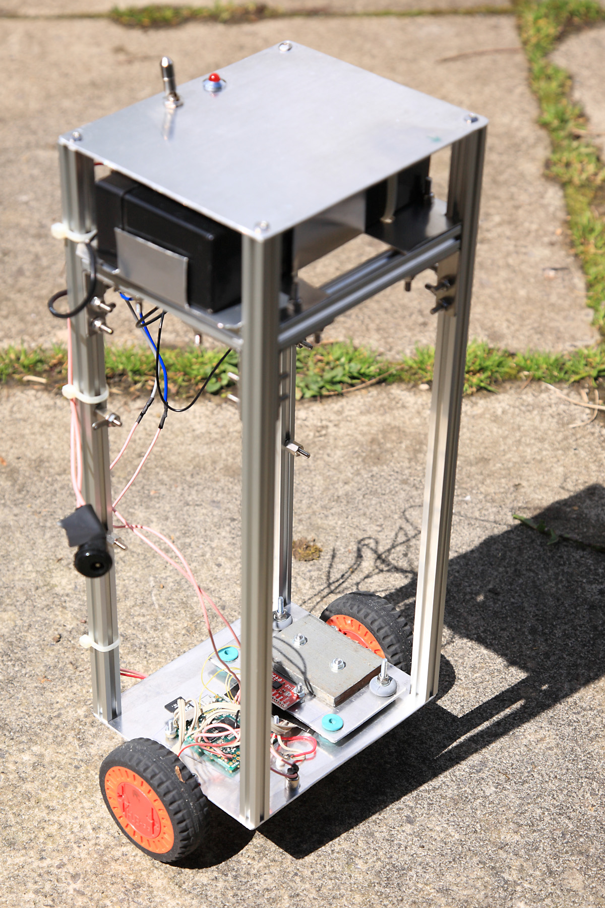
I've made a few changes to the algorithm which I thought I'd share to see what you think. These are intended as food for thought
and aren't intended as criticism. First a couple of minor points on program style.
The local gangle and global gangle variables are identical. To avoid this and to lose an unneccesary global, I have a local fangle
variable set to zero at the start of the main balance loop. The CF now looks like this
Code: Select all
def compf(fangle, accel,gyro,looptime,A):
    return A * (fangle + gyro * looptime/1000000) + (1-A) * accel
Secondly a neat way to implement a symmetrical constraint is
Code: Select all
def constrain(val, maxv):
    return min(maxv, max(-maxv, val))
As for the algorithm I wanted to simplify this already simple function further to help me get my elderly brain round how it works. In particular minimising the number of global "magic numbers" and processing blocks. The system has one inevitably nonlinear element which is the motor speed. This will be constrained by physics if not in code

It seemed to me that the additional constraint on the angle could be eliminated. The input demand speed must already be constrained outside the loop to be less than the motor's capability otherwise the 'bot will fall over

. This, with the fact that the output speed is constrained sets a limit on the error signal. Hence, with a suitably chosen value of KpS, the demand angle is also constrained. I therefore choose KpS to ensure that the output of speedcontrol() is within +=7 degrees and eliminate the explicit constraint:
Code: Select all
# Motor max is 377mm/s, max demand 300mm/s so max error 677mm/s
KpS = 0.01  # +-6.77 degrees
def speedcontrol(target, current):
    return KpS*(target - current)
KpS obviously affects loop gain which can be compensated for by the choice of the value of K. I've modified the stability routine to reduce the number of constants to two: K and Kd - this is just algebra, but K sets the proportional gain in conjunction with the previously chosen KpS. Kd sets the derivative. In opposition to my desire to reduce global constants I've added one, LOOPTIME. This is the time to complete a single loop (currently 5000uS). This is because I wanted to experiment with different delay values and at present the integrator and the fspeed filter are dependent on this. With an explicit value the loop parameters can be made independent of duration. So I now have:
Code: Select all
K = 5.0
Kd = 0.7
LOOPTIME = const(3000)                            # uS per loop
def stability(target,current,rate):
    error = target - current
    return K * (error - Kd*rate) * LOOPTIME/5000  # 5000 is nominal loop time
Obviously LOOPTIME can be eliminated once a value has been chosen, and my current view is that your existing 5000 is good.
On the subject of the first order low pass filter on fspeed I'm using the computed value of motor speed as a proxy for the actual speed: with lightly
loaded DC motors it's pretty accurate in the steady state. Measuring the actual speed is an option, but would introduce additional phase lags. I thought, at least initially, I'd avoid this in the interests of simplicity. So the question arose as to whether there is any point in filtering a computed value coming from an integrator. In practice I found the filter seemed to make the robot harder to stabilise, presumably because of the extra pole it introduces. So I removed it.
My main loop now looks like this - with the speed and turn control removed for clarity. Your code for movement and rotation works fine on my 'bot.
Code: Select all
def balance():
    start = pyb.micros()
    controlspeed = 0
    fspeed = 0
    demandspeed = 0
    fangle = 0.0
    while abs(fangle) < 45:  # give up if inclination angle >=15 degrees
        angle  = imu.pitch()
        rate   = imu.get_gy()
        fangle = compf(fangle, angle, rate, pyb.elapsed_micros(start)) # filtered angle
        start = pyb.micros()
        fspeed = (motor1.speed + motor2.speed)/2
        tangle  = speedcontrol(demandspeed, fspeed)      # Get target angle
        controlspeed += stability(tangle, fangle, rate)  # stability control
        motor1.speed = -controlspeed                     # set motor speed in mm/s
        motor2.speed = -controlspeed
        pyb.udelay(LOOPTIME - pyb.elapsed_micros(start))

    motor1.speed = 0                                     # stop and turn off motors
    motor2.speed = 0
motor.speed returns the demand speed constrained to +-377 (units are mm/s at the wheel rim)
As for performance, the code runs in about 550uS so pyb.udelay() is passed around 4.4mS every 5mS loop. As you suggested, this is regardless of whether the atan2() simplification is used. So I use atan2(). The Pyboard clearly offers scope for faster looping but benefits are minimal. I tried values from 2mS to 20mS: the bot continued to balance but positional stability started to degrade for longer loop times.
On a final note - and this is a big one - the thought occurred to me that ideally the loop would be executed as a callback on a timer running
at 5KHz. This would allow the Pyboard to do concurrent processing such as handling radio control or sensors, passing demand speed to the handler running in the background. Challenging, because callbacks can't use the heap. Thus we'd either need to do integer processing with its scaling issues or use the inline assembler for floating point. The MPU-9150 driver would need some adaptation as by default its get_gyro() and get_accel() methods use the heap. And there is the question of whether the underlying I2C routines use it. I'll investigate in due course.
<later> Some quick tests indicate that running as a timer callback is a non-starter. The MicroPython I2C driver uses the heap.
